Excel XLOOKUP vs VLOOKUP: Speed and Performance Compared
Excel's XLOOKUP replaces VLOOKUP in Office 365. Compare XLOOKUP, VLOOKUP, and INDEX with real benchmarks to see which formula is fastest. Data-driven analysis.

Table of Contents
CAUTION
Please note that this blog post was originally written in German. This translation is for your convenience. Despite my best efforts to ensure accuracy, there may be translation errors. I apologize for any discrepancies or misunderstandings resulting from the translation. I appreciate any corrections in the comments or via email.
Introduction
In this article, we delve into Excel’s XLOOKUP function, a new feature designed to replace the widely-used VLOOKUP formula. I’ll compare XLOOKUP with VLOOKUP and INDEX, focusing on their speed. I’ll also provide examples to highlight the differences between these functions.
Microsoft announced the XLOOKUP formula for Excel on August 28, 2019. This formula, intended to replace the VLOOKUP formula (one of Excel’s most popular formulas), is included in Microsoft Office 365 (Affiliate Link) and Excel 2016 (and newer) for Windows, as well as Microsoft Excel 2021 (and newer) for macOS.
When XLOOKUP became available in my Excel version, I started using it more frequently than VLOOKUP. For those curious about what VLOOKUP is or the differences between the two, examples will follow.
It’s important to note that the recipient of the Excel file should also have a current version of Excel installed, otherwise further processing would not be possible.
I’ve often read in various Excel forums or on Reddit that XLOOKUP is faster, hence one should stop using VLOOKUP. I accepted these statements without verification and shared them with my colleagues.
In this article, I aim to demonstrate how the XLOOKUP function differs from VLOOKUP and particularly investigate whether XLOOKUP is indeed faster.
Use Case Example
To test, I created a table with random data via Mockaroo. The table has three columns with 1,000 entries each. The first column contains a unique ID (from 1 to 1000), the second column a name, and the third one an annual salary (ranging from €95.52 to €280,000.00).
| id | name | salery |
|---|---|---|
| 1 | Ellene Otley | 45,488.00 € |
| 2 | Noell Jiggen | 28,307.64 € |
| 3 | Dolorita Proud | 49,755.88 € |
| … | … | … |
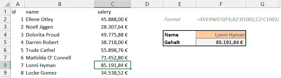
Now, I want to use a formula to search the table to find out how much money the fictional person Melody Waterhouse earns.
VLOOKUP
Since the first version of Excel, VLOOKUP can be used.
=VLOOKUP(lookup_value, table_array, col_index_num, [range_lookup])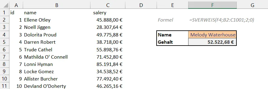
In my case, I use the formula as follows.
=VLOOKUP("Melody Waterhouse",{range with names and salary},2,0)The formula searches in the first column of the lookup range for the desired name and then returns the second column. By adding a 0 at the end, I set an exact match.
Issues can arise if you forget the 0 as the last argument. It can also be inconvenient if you have many columns. The search can only be done from left to right. If the salary were to the left of the name, the formula would not work. If the salary were below the name, you would have to use the HLOOKUP function instead to search from top to bottom.
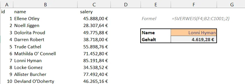
In my opinion, having the inexact search set as default is a design flaw. In this case, I don’t even understand why the person at id 1 is not displayed, after all, L lies alphabetically between E and N.
INDEX / MATCH
In the past, when I wanted more customization options, I often resorted to the combination of the INDEX and MATCH formulas.
=INDEX(array,row_num,column_num)
=MATCH(lookup_value,lookup_array,match_type)
=INDEX(array,MATCH(lookup_value,lookup_array,match_type),column_num)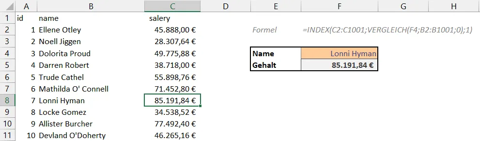
With the INDEX formula, I enter the array from which I want to retrieve information (in my case the column with the salaries). I don’t know the absolute row, so it is searched with the MATCH formula.
Advantages:
- Search from right to left and from bottom to top possible
Disadvantages:
- Formula readability is more difficult
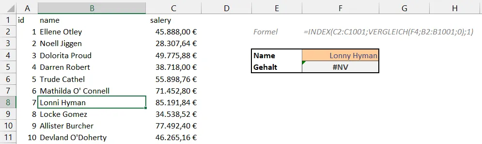
As with VLOOKUP, an error is returned if the name cannot be found.
XLOOKUP
The new XLOOKUP function solves some of the limitations of the other formulas.
=XLOOKUP(lookup_value,lookup_array,return_array,if_not_found,match_mode,search_mode)The first three arguments must be specified, the rest are optional.
Here, the use is more or less self-explanatory.
Advantages:
- Easiest use
- Built-in “not found” argument
- Exact match set by default
- Various comparison modes
- Search direction adjustable, as search and return arrays can be specified separately
Disadvantages:
- Compatibility
Behavior with Unfound Entries
As mentioned earlier, XLOOKUP has an integrated parameter to return a different value when an entry is not found.
When using INDEX or VLOOKUP, you can only fall back on the IFERROR formula.
=IFERROR(value,value_if_error)Speed Measurement
Now I am interested in the speed of the lookup possibilities.
To measure speed, I followed Microsoft’s documentation.
So I created a new module with the following code.
Private Declare PtrSafe Function getFrequency Lib "kernel32" Alias _
        "QueryPerformanceFrequency" (cyFrequency As Currency) As Long
Private Declare PtrSafe Function getTickCount Lib "kernel32" Alias _
         "QueryPerformanceCounter" (cyTickCount As Currency) As Long

Function Microtimer() As Double
'

' Returns seconds.
    Dim cyTicks1 As Currency
    Static cyFrequency As Currency
    '
    Microtimer = 0

' Get frequency.
    If cyFrequency = 0 Then getFrequency cyFrequency

' Get ticks.
    getTickCount cyTicks1

' Seconds
    If cyFrequency Then Microtimer = cyTicks1 / cyFrequency
End Function

Sub RangeTimer()
    DoCalcTimer 1
End Sub
Sub SheetTimer()
    DoCalcTimer 2
End Sub
Sub RecalcTimer()
    DoCalcTimer 3
End Sub
Sub FullcalcTimer()
    DoCalcTimer 4
End Sub

Sub DoCalcTimer(jMethod As Long)
    Dim dTime As Double
    Dim dOvhd As Double
    Dim oRng As Range
    Dim oCell As Range
    Dim oArrRange As Range
    Dim sCalcType As String
    Dim lCalcSave As Long
    Dim bIterSave As Boolean
    '
    On Error GoTo Errhandl

' Initialize
    dTime = Microtimer

    ' Save calculation settings.
    lCalcSave = Application.Calculation
    bIterSave = Application.Iteration
    If Application.Calculation <> xlCalculationManual Then
        Application.Calculation = xlCalculationManual
    End If
    Select Case jMethod
    Case 1

        ' Switch off iteration.

        If Application.Iteration <> False Then
            Application.Iteration = False
        End If

        ' Max is used range.

        If Selection.Count > 1000 Then
            Set oRng = Intersect(Selection, Selection.Parent.UsedRange)
        Else
            Set oRng = Selection
        End If

        ' Include array cells outside selection.

        For Each oCell In oRng
            If oCell.HasArray Then
                If oArrRange Is Nothing Then
                    Set oArrRange = oCell.CurrentArray
                End If
                If Intersect(oCell, oArrRange) Is Nothing Then
                    Set oArrRange = oCell.CurrentArray
                    Set oRng = Union(oRng, oArrRange)
                End If
            End If
        Next oCell

        sCalcType = "Calculate " & CStr(oRng.Count) & _
            " Cell(s) in Selected Range: "
    Case 2
        sCalcType = "Recalculate Sheet " & ActiveSheet.Name & ": "
    Case 3
        sCalcType = "Recalculate open workbooks: "
    Case 4
        sCalcType = "Full Calculate open workbooks: "
    End Select

' Get start time.
    dTime = Microtimer
    Select Case jMethod
    Case 1
        If Val(Application.Version) >= 12 Then
            oRng.CalculateRowMajorOrder
        Else
            oRng.Calculate
        End If
    Case 2
        ActiveSheet.Calculate
    Case 3
        Application.Calculate
    Case 4
        Application.CalculateFull
    End Select

' Calculate duration.
    dTime = Microtimer - dTime
    On Error GoTo 0

    dTime = Round(dTime, 5)
    MsgBox sCalcType & " " & CStr(dTime) & " Seconds", _
        vbOKOnly + vbInformation, "CalcTimer"

Finish:

    ' Restore calculation settings.
    If Application.Calculation <> lCalcSave Then
         Application.Calculation = lCalcSave
    End If
    If Application.Iteration <> bIterSave Then
         Application.Iteration = bIterSave
    End If
    Exit Sub
Errhandl:
    On Error GoTo 0
    MsgBox "Unable to Calculate " & sCalcType, _
        vbOKOnly + vbCritical, "CalcTimer"
    GoTo Finish
End Sub
Now I have the ability to recalculate a workbook or completely recalculate it and display how long it took.
In particular, I used the function with Application.CalculateFull, but also tried Application.Calcuate.
Test 1 - Calculate 100,000 Cells
Test 1 - Setup
For the first test, I created a new workbook. One worksheet contains data in two columns. One of them contains the ID, and the other a random number between 0 and 1:
| ID | Wert |
|---|---|
| 1 | 0.97714411 |
| 2 | 0.57334089 |
| 3 | 0.86522436 |
| … | … |
| 100000 | 0.04843126 |
On another worksheet, I copied the 100,000 rows with the ID and tried to retrieve the corresponding value via different lookup methods.
The test device is a laptop with an AMD Ryzen 4600H CPU.
Results of Test 1
First, I used RangeTimer and checked how long it took to calculate each column. This did not work so well. In contrast to VLOOKUP, whose area took about 0.06 seconds for the update, the INDEX/MATCH combination took about 64 seconds and XLOOKUP over two minutes. So I started creating separate files and repeatedly performed a complete recalculation and compared the average duration:
I wondered if I was doing something wrong because XLOOKUP was significantly slower than the other two lookup methods. I tried it again with a Surface (Intel Core i5 Gen 8 CPU). I came to a very similar result:
This hypothesis that XLOOKUP has better performance could not be verified. So I tried to vary the test.
Here I tried using RecalcTimer (i.e., not a complete recalculation):
AMD:
INTEL:
By the way, this does not constitute a comparison between Intel and AMD CPUs per se; the two devices are completely different.
Unless otherwise stated, I will use FullcalcTimer in what follows because I want to know how long it takes in a worst-case scenario.
There was no measurable difference in performance here either. So I changed the test again. I changed the 100 on the first worksheet to 1,000,000 in my worksheet. As a result, the value belonging to 100 could no longer be found in the second sheet:
AMD:
Intel:
The strange thing is that the entire calculation works much faster due to the error. XLOOKUP was still slower than the other formulas, although this time imperceptibly so.
Next, I tried to correct the error against an empty field. For XLOOKUP with the built-in parameter and for the other two formulas with an additional IFERROR query:
AMD:
Intel:
Overall, XLOOKUP didn’t seem to be any faster, so I converted the test again.
2D Lookup
The great thing about lookup formulas is that it is also possible to search with a variable column index. Let’s assume we have a price list of a coffee shop:
| Beverage | Tall | Grande | Venti |
|---|---|---|---|
| Caffè Americano | 3.39 | 3.89 | 4.39 |
| Caffè latte | 3.99 | 4.59 | 4.99 |
| Earl Gray | 2.69 | 3.19 | 3.69 |
| Coffee Frapuccino | 4.79 | 5.29 | 5.79 |
| Iced White Chocolate Mocha | 4.99 | 5.49 | 5.99 |
Now we don’t want to pivotize the table but get the price directly by specifying the beverage and size.
2D Lookup with INDEX / MATCH
With INDEX, we can specify the column as a third parameter. We want to find out how expensive the Caffè Americano is in Venti size.
=INDEX(A1:D6, 2, 4)
or
=INDEX(B2:D6, 1, 3)
But we don’t necessarily know that Caffè Americano is at the top position. Therefore we need the MATCH formula:
=INDEX(A1:D6, MATCH("Caffé Americano", A1:A6, 0), 3)
oder
=INDEX(B2:D6, MATCH("Caffé Americano", A2:A6, 0), 3)
Now we also don’t know that Venti is all the way to the right, so that needs replacing too:
=INDEX(A1:D6, MATCH("Caffé Americano", A1:A6, 0), MATCH("Venti", A1:D1, 0))
or
=INDEX(B2:D6, MATCH("Caffé Americano", A2:A6, 0), MATCH("Venti", B1:D1, 0))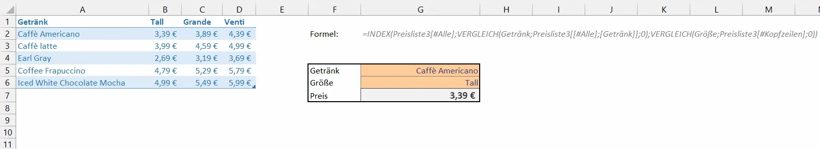
2D Lookup with VLOOKUP
With VLOOKUP, additional functionality can be added only through MATCH. Normally we would enter the following formula:
=VLOOKUP("Caffè Americano", A1:D6, 4, 0)We can search for the correct column (in this case “4”) with MATCH:
=VLOOKUP("Caffè Americano", A1:D6, MATCH("Venti", A1:D1, 0), 0)2D Lookup with XLOOKUP
With XLOOKUP, basic search works as follows:
=XLOOKUP("Caffè Americano", A1:A6, D1:D6)
or
=XLOOKUP("Caffè Americano", A2:A6, D2:D6)
But the return array must be able to shift variably. At this point we simply use a second XLOOKUP formula
=XLOOKUP(Beverage,A2:A6,XLOOKUP(Size,B1:D1,B2:D6))
in a table:
=XLOOKUP(Beverage,PriceList[Beverage],XLOOKUP(Size,PriceList[[#Headers],[Tall]:[Venti]],PriceList[[Tall]:[Venti]]))
Test 2 - 2D Lookup
Test 2 - Setup
Here I took the same setup as in Test 1 but added four more columns.
| ID | 1 | 2 | 3 | 4 | 5 |
|---|---|---|---|---|---|
| 1 | 0.97714411 | 0.34313251 | 0.47387243 | 0.92325136 | 0.70448042 |
| 2 | 0.57334089 | 0.59227904 | 0.72094532 | 0.62649883 | 0.10888043 |
| … | … | … | … | … | … |
| 100000 | 0.04843126 | 0.44973681 | 0.49224276 | 0.37683903 | 0.03069793 |
The table on the second sheet received an additional column with an integer between 1 and 5. The goal was then to find the value in each respective column.
| ID | Column | Formula |
|---|---|---|
| 1 | 1 | =FORMULA |
| 2 | 2 | =FORMULA |
| 3 | 1 | =FORMULA |
| 4 | 3 | =FORMULA |
| 5 | 3 | =FORMULA |
| … | … | … |
| 100000 | 4 | =FORMULA |
Results of Test 2
I repeatedly performed a complete recalculation and compared the average duration of each method:
AMD:
INTEL:
Again, XLOOKUP could not outperform VLOOKUP or INDEX/MATCH in terms of performance.
Test 3 - Unsorted data
Test 3 - Setup
For the third test, I generated new sample data.
| id | first_name | last_name | gender | ip_address | |
|---|---|---|---|---|---|
| 1 | Andee | Audibert | aaudibert0@jigsy.com | Female | 139.9.209.124 |
| 2 | Kaitlyn | Bollard | kbollard1@chronoengine.com | Female | 32.192.138.202 |
| … | … | … | … | … | … |
| 1000 | Layton | Geely | lgeely7@pen.io | Agender | 193.33.184.242 |
Results of Test 3
Then on another sheet, I tried to find the IP address via ID. From here on out, I only used the AMD laptop because any relative differences between devices were negligible.
Then I searched for email addresses via ID but as a two-dimensional search this time..
Again here XLOOKUP was unfortunately not faster than other methods. When using RecalcTimer, XLOOKUP had better values but all numbers are very small where even a slight delay due to an external factor plays a larger role.
Then I wondered if there might be a difference whether I search in an ordered row or not. Therefore, I took the previously generated fictitious email addresses and sorted them alphabetically. I then searched for the IP address in the original list. This time, I tried recalculating with the RangeTimer.
Disappointingly, XLOOKUP was significantly slower in recalculating.
Test 4 - Approximate Match Mode
Setup
However, there is also an alternative match mode, which is set by default in VLOOKUP. I wanted to try this as well.
I took my initial data (ID, Name, Annual Income) and aimed to calculate it according to § 32a EStG.
I did this quite awkwardly by creating three new columns named “x”, “y”, and “z”.
x:
=ROUNDDOWN(AnnualIncome, 0)
y:
=MAX((x-9984)/10000, 0)
z:
=MAX((x-14926)/10000, 0)
Then, in another area, I created additional data. It is important that the data in the lookup column (in my case taxable income) are sorted in ascending order:
| taxable_income | Index |
|---|---|
| 0 | 0 |
| 9985 | 1 |
| 14927 | 2 |
| 58597 | 3 |
| 277826 | 4 |
This allowed me to choose which formula to use for the calculation, in the example of VLOOKUP as follows.
=SWITCH(
    VLOOKUP(
        {AnnualIncome},
        {Second data range},
        2,
        1
    ),
    0,
    0,
    1,
    (1008.7*y+1400)*y,
    2,
    (206.43*z+2397)*z+938.24,
    3,
    0.42*x-9267.53,
    4,
    0.45*x-17602.28
)
What happens here? VLOOKUP looks for the formula index in the second data range. For example, Ellene Otley in my sample data has an income of €45,888. Now VLOOKUP looks for this in the other area but with the approximate match mode. VLOOKUP checks if the number is greater than or equal to 9985. Then, if the number is greater than or equal to 14,927. After that, if the number is greater than or equal to 58,597. 45,888 is less than 58,597, so VLOOKUP steps back and returns “2” from the second column.
With XLOOKUP, I can then define what should happen when a 2 is returned.
=SWITCH(
    {Here I use one of the match functions and get a number between 0 and 4},
    0,
    {What should happen when 0 is returned},
    1,
    {What should happen when 1 is returned},
    and so on.
)
This results in €10,338.76 for an annual income of €45,888. This means that with an annual income of €45,888 you pay approximately 23% income tax.
Results of the fourth test
Here too, the XLOOKUP function was not faster than the other methods. With RecalcTimer, XLOOKUP had better values, but all numbers are very small. A slight delay due to an external factor plays a bigger role.
Then I wondered if moving the columns “x”, “y”, and “z” directly into the formula would make a difference. I deleted these three columns and adjusted the tax calculation formula.
=LET(
    x,
    ABRUNDEN({AnnualIncome},0),
    y,
    MAX((x-9984)/10000,0),
    z,
    MAX((x-14926)/10000,0),
    SWITCH(
        {as before}
    )
)
The results here are again very similar. Also with RecalcTimer:
Then I compared it by completely removing the reference and integrating it into the formula to see if this makes the calculation faster:
=LET(
    taxable_income,
    {AnnualIncome},
    x,
    ROUNDDOWN(taxable_income,0),
    y,MAX((x-9984)/10000,0),
    z,
    MAX((x-14926)/10000,0),
    SWITCH(
        TRUE,
        taxable_income<9985,
        0,
        taxable_income<14927,
        (1008.7*y+1400)*y,
        taxable_income<58597,
        (206.43*z+2397)*z+938.24,
        taxable_income<277826,0.42*x-9267.53,
        0.45*x-17602.28
    )
)
This pushed the entire recalculation down to an average of 0.00937 seconds. With RecalcTimer, it was 0.0002 seconds. This shows that a lookup function is not always the best solution.
Returning Multiple Values
For the sake of completeness, I would also like to mention that it is possible to return multiple values with functions in Excel. The FILTER function can be used for this.
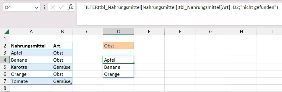
In this example, I receive the fruit as a matrix.
If I want all the values in one cell, I can combine the function with the TEXTJOIN function.
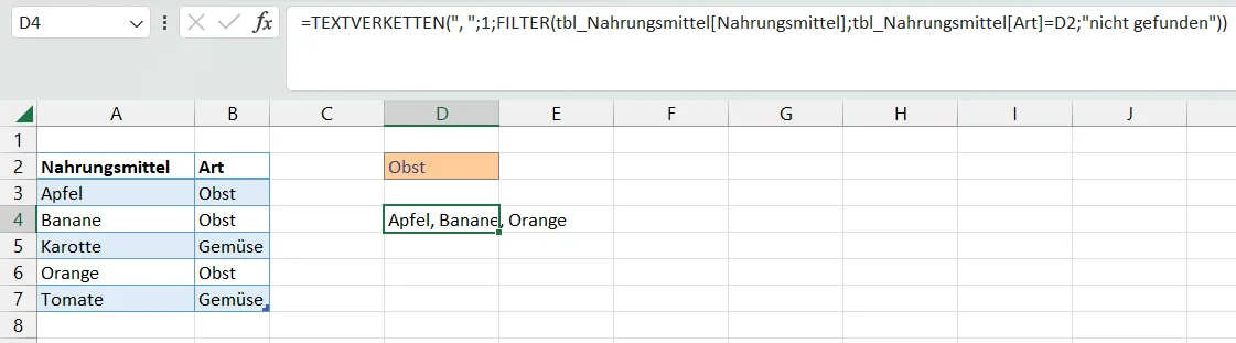
=TEXTJOIN(", ", TRUE, FILTER(tbl_Food[Food], tbl_Food[Type]=D2, "not found"))Conclusion
I could not confirm the assumption that the XLOOKUP function is faster than the VLOOKUP function. On the contrary, it seemed that XLOOKUP was slower than INDEX or VLOOKUP. Does this mean that I recommend using VLOOKUP? No, especially not when you need the additional arguments of XLOOKUP. Furthermore, in most normal use cases, the difference will hardly be noticeable. I am just showing that there can still be use cases where it makes sense to use VLOOKUP and also want to refute the claim that XLOOKUP is the faster formula.
Related Articles
Excel VLOOKUP Function Tutorial - Use VLOOKUP in Excel
The VLOOKUP function in Excel explained simply: Learn how to reliably search data in tables, apply the formula correctly, and discover useful alternatives.
Combine and Pivot Text Data in Excel Using PowerQuery
Combine text columns and pivot datasets in Excel using PowerQuery. Learn how to merge and transform data efficiently with practical examples. Step-by-step tutorial.
Excel: Group and Sort Table Data Dynamically with Formulas
Group and sort data from an Excel table dynamically using formulas. No pivot tables needed, so you keep full control over your data analysis and evaluations.
PostgreSQL vs. MariaDB vs. SQLite: A Performance Test
Which database fits your project best? A detailed performance benchmark comparing PostgreSQL, MariaDB, and SQLite with practical recommendations for your setup.