Excel VLOOKUP Function Tutorial - Use VLOOKUP in Excel
The VLOOKUP function in Excel explained simply: Learn how to reliably search data in tables, apply the formula correctly, and discover useful alternatives.

Table of Contents
CAUTION
Kindly note, this blog post was initially written in German and has been translated for your convenience. Despite my best efforts to maintain accuracy, there might be translation errors. I apologize for any discrepancies or misunderstandings that may arise from the translation and appreciate any corrections in the comments or via email.
Microsoft Excel offers a myriad of functions for data analysis. Among the most renowned is the VLOOKUP function, which is instrumental in identifying data within tables. This guide simplifies the use of the VLOOKUP function in Excel, demonstrating how to search for data in tables and introducing alternatives.
Understanding the VLOOKUP Function in Excel
VLOOKUP, or Vertical Lookup, is a frequently used Excel command, particularly useful when dealing with large data sets. This command enables users to locate and extract specific values from a table or column by specifying a reference cell and a column to search. For instance, if you have a table comprising two columns (Name and Email Address), you can employ the VLOOKUP command to search for a specific name and retrieve the corresponding email address.
However, remember that VLOOKUP searches exclusively from left to right.
Syntax of the VLOOKUP Formula
The syntax for the VLOOKUP formula is as follows:
=VLOOKUP(lookup_value, table_array, col_index_num, [range_lookup])Parameters
-
Lookup_value: The value to be searched in the first column of the table array. This value can be text, a logical value, or a number.
-
Table_array: The range where the lookup and return values are stored. This range must contain at least two columns.
-
Col_index_num: The column in the table array from which the value should be returned. The first column (from the left side) in the table array is represented by col_index_num 1. The next right column is represented by the column index number 2, and so on.
-
Range_lookup: A logical value specifying whether you want an exact or approximate match. TRUE or 1 performs an approximate match. FALSE or 0 performs an exact match. If the range_lookup argument is omitted, an approximate match is performed.
Practical Examples of the VLOOKUP Function
Here are some examples of using the VLOOKUP function in Excel.
Basic VLOOKUP Function
Let’s start with a table containing names and email addresses.
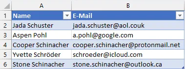
Suppose I want to find the email address of “Cooper Schinacher.” I can use the VLOOKUP function for this.
=VLOOKUP("Cooper Schinacher",A2:B6,2,FALSE)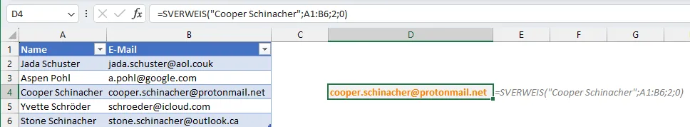
I can also format the range A1:B6 as a table (CTRL+T) and use the table as a table_array.
=VLOOKUP("Cooper Schinacher",Table1,2,FALSE)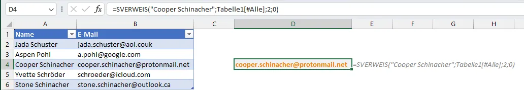
Dynamic Column Index
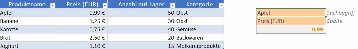
Next, I have a table about inventory stock, with Product, Price, Quantity, and Category. I can find out how expensive an apple is by using the VLOOKUP.
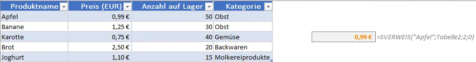
=VLOOKUP("Apple",A2:D6,2,FALSE)But what if I’m unsure about the column containing the price? I can make the column index dynamic by using the MATCH function.
=VLOOKUP("Apple",A2:D6,MATCH("Price (EUR)",A1:D1,0),FALSE)
or
=VLOOKUP("Apple",Table2,MATCH("Price (EUR)",Table2[#Headers],0),FALSE)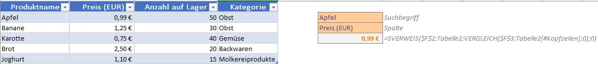
Handling Nonexistent Lookup Value
If the lookup value does not exist, VLOOKUP returns the error #N/A.
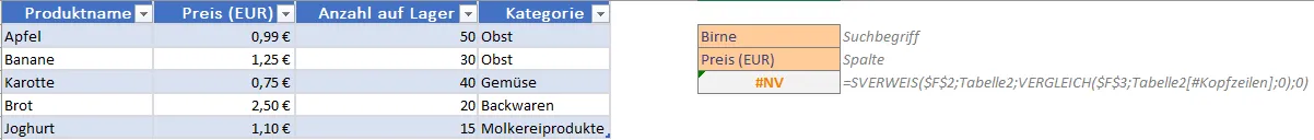
This can be managed with the IFNA function.
=IFNA(VLOOKUP("Pear",A2:D6,2,FALSE),"Not found")
However, it’s not ideal now because it’s unclear whether the product or the column name doesn’t exist. But I can address this with the IF and ISNA functions.
=IFNA(VLOOKUP($F$2,Table2,MATCH($F$3,Table2[#Headers],0),FALSE),IF(ISNA(MATCH($F$3,Table2[#Headers],0)),"Column not found","Product not found"))It’s even simpler when parts of the function are defined with LET.
=LET(Lookup_value,$F$2,Table,Table2,Headers,Table2[#Headers],Column_name,$F$3,Col_index,MATCH(Column_name,Headers,0),
IFNA(VLOOKUP(Lookup_value,Table,Col_index,FALSE),IF(ISNA(Col_index),"Column not found","Product not found")))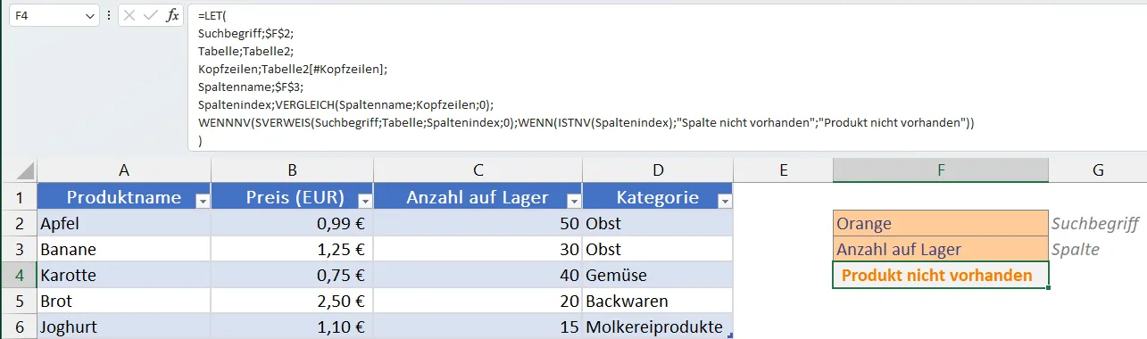
By the way, you should also make sure that the types of the search criteria and the matrix match. For example, if I search for “1” (text), VLOOKUP will only find a “1” (as text) and not 1 (as a number). Accordingly, for numbers it is a good idea to use the VALUE function beforehand, to ensure that the types match. This can also be checked with the TYPE formula.
Search Across Multiple Worksheets
Suppose I have an Excel file with several worksheets. On each worksheet, I have a table with products and prices.
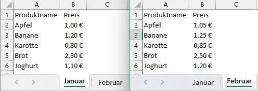
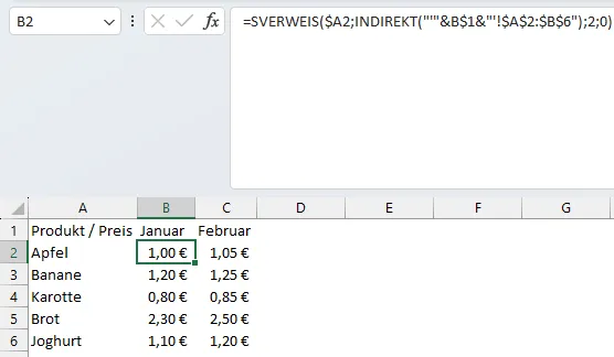
Now, I want to summarize the prices for January and February in one table. For this, I use the VLOOKUP function together with the INDIRECT function.
=VLOOKUP($A2,INDIRECT("'"&B$1&"'!$A$2:$B$6"),2,FALSE)In this way, I dynamically switch the worksheet in the VLOOKUP function.
Approximate Match
In some cases, an approximate match is also needed.
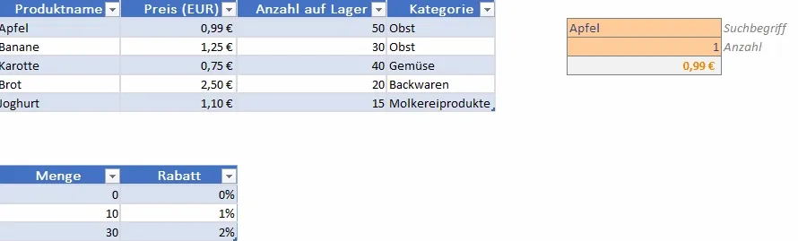
I have a table with products and prices (tbl_Products) and a second table with a quantity discount (tbl_QuantityDiscount).

=LET(
Lookup_value,$F$2,
Table,tbl_Products,
Quantity,$F$3,
IFNA(VLOOKUP(Lookup_value,Table,2,FALSE)*Quantity,"Product not found")
)
However, if the quantity exceeds 10, the price should be discounted using the data from the tbl_QuantityDiscount table.
Here, I need the approximate match because the quantity could be not only 10 but also, for example, 11.
=LET(
Lookup_value,$F$2,
Quantity,$F$3,
Discount,1-VLOOKUP(Quantity,tbl_QuantityDiscount,2,TRUE),
IFNA(VLOOKUP(Lookup_value,tbl_Products,2,FALSE)*Quantity*Discount,"Product not found")
)
VLOOKUP with Multiple Criteria
In some cases, you need to search for multiple criteria. In this case you have to combine the VLOOKUP function with the CHOOSE formula.
For example, you have a table with data from balance sheets of multiple companies.
| / | A | B | C | D |
|---|---|---|---|---|
| 1 | Company | Year | Position | Value |
| 2 | Company A | 2019 | Assets | 100 |
| 3 | Company A | 2019 | Liabilities | 50 |
| 4 | Company A | 2020 | Assets | 120 |
| 5 | Company A | 2020 | Liabilities | 60 |
| 6 | Company B | 2019 | Assets | 200 |
| 7 | Company B | 2019 | Liabilities | 100 |
| 8 | Company B | 2020 | Assets | 240 |
| 9 | Company B | 2020 | Liabilities | 120 |
Now you want to find the value of the assets of Company A in 2020. For this you can use the following formula:
=VLOOKUP("Company A" & "-" & "2020" & "-" & "Assets",CHOOSE({1,2},A2:A9 & "-" & B2:B9 & "-" & C2:C9,D2:D9),2,FALSE)What happens here? The CHOOSE function creates a new array with the company name, year and position combined in one column and the value in the second column. The VLOOKUP function then searches for the same combination of the company name, year and position and returns the value (column 2).
Alternatives to VLOOKUP
Searching Downwards
The VLOOKUP function constantly searches to the right. If I want to search horizontally (downwards), I can use the HLOOKUP function.
=HLOOKUP(Lookup_value, Table_array, Row_index_num, [Range_lookup])INDEX and MATCH
I can use the INDEX and MATCH functions for more flexibility regarding the search direction and column selection.
=INDEX(Table_array,MATCH(Lookup_value, Table_array,[Match_type]),[Col_index_num])XLOOKUP
Since 2019, Excel has integrated the XLOOKUP formula, which can replace VLOOKUP, HLOOKUP, Index and Match. The function includes a search function in all directions and integrated error handling. However, you should consider compatibility issues with older Excel versions and the speed for larger file quantities.
=XLOOKUP(Lookup_value, Lookup_array, Return_array, if_not_found, Match_mode, Search_mode)In the long run, VLOOKUP will probably be replaced by XLOOKUP because it offers more possibilities and is easier to handle.
SUMIFS
A possible problem with VLOOKUP is that it only returns the first match. If I want to calculate the sum of fruit items in stock, SUMIFS can consider and sum all matches.
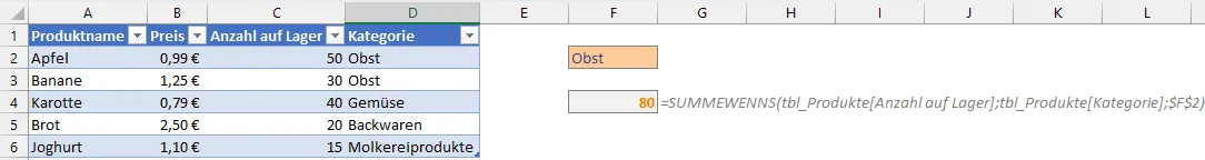
=SUMIFS(tbl_Products[Quantity in stock],tbl_Products[Category],$F$2)Combined with the COUNTIFS function, I can also determine the number of matches.
=TEXTJOIN(": ",0,COUNTIFS(tbl_Products[Category],$F2),SUMIFS(tbl_Products[Quantity in stock],tbl_Products[Category],$F2))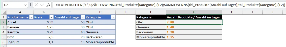
Filter
If I want to see all matches, I can also use the new FILTER function. In my case, I combine it with the TRANSPOSE function to display the results in a row.
=TRANSPOSE(FILTER(tbl_Products[Product name],tbl_Products[Category]=$F2))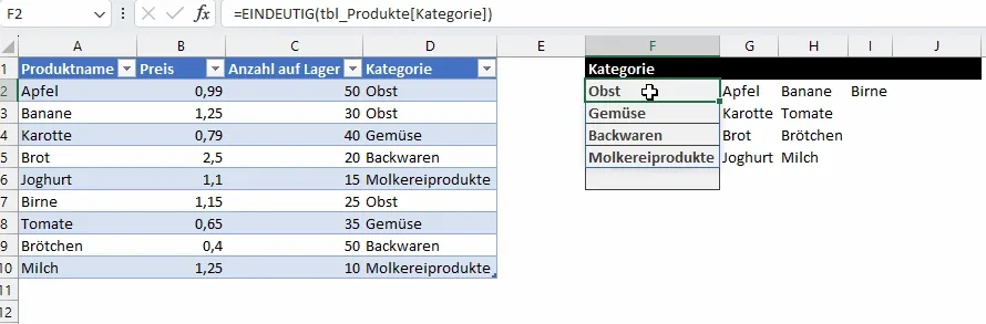
Wrapping Up
While VLOOKUP is a highly popular function in Excel, there are numerous alternative methods that might be better suited depending on the situation. The choice of the right method depends on the type of data and the specific requirements of the evaluation. Therefore, it’s worthwhile to experiment with different approaches to find out which is best suited for your needs.
What is the VLOOKUP function in Excel?
How do I use VLOOKUP in Excel?
Can VLOOKUP return text values?
How does column index number work in VLOOKUP?
What is the difference between VLOOKUP and HLOOKUP?
How do I use the VLOOKUP function across multiple sheets?
Why did my VLOOKUP return #N/A?
Why do I have to search for the lookup value in the first column of the table array?
Why is my VLOOKUP not working?
Related Articles
Excel XLOOKUP vs VLOOKUP: Speed and Performance Compared
Excel's XLOOKUP replaces VLOOKUP in Office 365. Compare XLOOKUP, VLOOKUP, and INDEX with real benchmarks to see which formula is fastest. Data-driven analysis.
Excel: Group and Sort Table Data Dynamically with Formulas
Group and sort data from an Excel table dynamically using formulas. No pivot tables needed, so you keep full control over your data analysis and evaluations.
Combine and Pivot Text Data in Excel Using PowerQuery
Combine text columns and pivot datasets in Excel using PowerQuery. Learn how to merge and transform data efficiently with practical examples. Step-by-step tutorial.