Excel: Group and Sort Table Data Dynamically with Formulas
Group and sort data from an Excel table dynamically using formulas. No pivot tables needed, so you keep full control over your data analysis and evaluations.

Table of Contents
Excel offers many possibilities for analyzing and preparing table data. Especially with larger amounts of data, it is often helpful to group and sort the data according to certain criteria to get a better overview.
In my daily work with Excel, I often encounter situations where I need to clearly present and evaluate data. The standard functions are not always sufficient for this. Especially when the grouped data should be displayed below each other on a worksheet, you quickly reach limits with built-in tools like pivot tables or the Power Query Editor.
That’s why I looked for a solution to flexibly group table data with formulas. The data should be dynamically summarized based on the values in the first column. Within the groups, you should be able to sort the rows individually.
Perhaps this task will become easier with the introduction of the GROUPBY function. However, this formula is only available in the beta channel of Excel.
After some research, I came across an interesting solution on Reddit that served as a starting point. I adapted the formula and now want to share it here on my blog.
In the following, I show how the formula is structured and which Excel functions are used. Using a practical example, I explain how to apply the formula.
Requirements
- Microsoft 365 (Amazon Affiliate-Link)
Source Table
The formula should group the data from a table (or range) based on the first column.
Let’s assume we have the following table:
| Kaffeesorte | Herkunft | Röstgrad | Preis/kg | Bewertung |
|---|---|---|---|---|
| Arabica | Kolumbien | mittel | 28,00 € | 4,5 |
| Robusta | Vietnam | dunkel | 18,00 € | 3,8 |
| Arabica | Äthiopien | hell | 32,00 € | 4,8 |
| Liberica | Philippinen | mittel | 24,00 € | 4,2 |
| Arabica | Brasilien | mittel | 26,00 € | 4,4 |
| Robusta | Indonesien | dunkel | 20,00 € | 4,0 |
| Arabica | Kenia | hell | 30,00 € | 4,7 |
| Excelsa | Südostasien | dunkel | 22,00 € | 4,1 |
| Arabica | Guatemala | mittel | 29,00 € | 4,6 |
| Robusta | Uganda | mittel | 19,00 € | 3,9 |
| Arabica | Costa Rica | hell | 31,00 € | 4,9 |
| Liberica | Malaysia | dunkel | 23,00 € | 4,3 |
| Arabica | Jamaika | mittel | 35,00 € | 5,0 |
Goal
The formula should group the data by coffee type. Within the groups, the rows are sorted individually. The result should look something like this:
| Kaffeesorte | |||
|---|---|---|---|
| Arabica | |||
| Herkunft | Röstgrad | Preis/kg | Bewertung |
| Jamaika | mittel | 35,00 € | 5,0 |
| Costa Rica | hell | 31,00 € | 4,9 |
| Äthiopien | hell | 32,00 € | 4,8 |
| Kenia | hell | 30,00 € | 4,7 |
| Guatemala | mittel | 29,00 € | 4,6 |
| Kolumbien | mittel | 28,00 € | 4,5 |
| Brasilien | mittel | 26,00 € | 4,4 |
| Robusta | |||
| Herkunft | Röstgrad | Preis/kg | Bewertung |
| Indonesien | dunkel | 20,00 € | 4,0 |
| Uganda | mittel | 19,00 € | 3,9 |
| Vietnam | dunkel | 18,00 € | 3,8 |
| Liberica | |||
| Herkunft | Röstgrad | Preis/kg | Bewertung |
| Malaysia | dunkel | 23,00 € | 4,3 |
| Philippinen | mittel | 24,00 € | 4,2 |
| Excelsa | |||
| Herkunft | Röstgrad | Preis/kg | Bewertung |
| Südostasien | dunkel | 22,00 € | 4,1 |
Explanation of Used Excel Functions
To achieve this, several formulas are needed.
UNIQUE
Returns a list of the unique values in a range or array.
=UNIQUE(A1:A10)Returns a list of unique values from the range A1:A10.
| A |
|---|
| Apple |
| Pear |
| Apple |
| Banana |
| Pear |
Result:
| Unique Values |
|---|
| Apple |
| Pear |
| Banana |
SWITCH
Compares a value to a list of values and returns the first result that matches the condition.
=SWITCH(A1=1,"Yes",A1=0,"No",TRUE,"Unknown")Compares the value in A1 to 1 and returns “Yes” if equal, “No” if 0, and “Unknown” for all other values.
FILTER
Filters an array based on a condition and returns the resulting array.
=FILTER(A1:A5,A1:A5>3)Returns all values in the range A1:A5 that are greater than 3.
| A |
|---|
| 1 |
| 5 |
| 2 |
| 7 |
| 3 |
Result:
| Filtered Values |
|---|
| 5 |
| 7 |
LAMBDA
Defines a named function that can be used in other formulas.
=LAMBDA(x, x * 2)(5)Defines a function that multiplies the argument x by 2 and returns the result for x=5 (10).
LET
Defines a function that multiplies the argument x by 2 and returns the result for x=5 (10).
=LET(x, 5, y, 10, x+y)Result: 15. The variables x and y are defined within the LET function and can be used in the calculation.
INDEX
Returns a value or reference to a value at a specific position in a range or array.
=INDEX(A1:C5, 2, 3)Returns the value in the second row and third column of the range A1:C5.
| A | B | C |
|---|---|---|
| 1 | 2 | 3 |
| 4 | 5 | 6 |
| 7 | 8 | 9 |
Result: 6.
MAP
Applies a function to each element of an array and returns the resulting array.
=MAP(A1:A5, LAMBDA(x, x * 2))Multiplies each element in the range A1:A5 by 2.
| A |
|---|
| 1 |
| 5 |
| 2 |
| 7 |
| 3 |
Result:
| Doubled Values |
|---|
| 2 |
| 10 |
| 4 |
| 14 |
| 6 |
MAKEARRAY
Creates an array based on the specified dimensions and a lambda function.
=MAKEARRAY(3, 3, LAMBDA(row, col, row * col))Creates a 3x3 array where each element is the product of the row and column index.
MAX
Returns the largest number in a set of values.
=MAX(A1:A5)Returns the largest value in the range A1:A5.
MOD
Returns the remainder of a division.
=MOD(10, 3)Returns the remainder of dividing 10 by 3 (1).
SCAN
Performs a calculation for each element of an array and returns a cumulative result.
=SCAN(0, A1:A5, LAMBDA(cumulative, value, cumulative + value))Calculates the cumulative sum of the values in the range A1:A5.
SEQUENCE
Creates an array of sequential numbers based on the specified parameters.
=SEQUENCE(5, 1, 1, 1)Creates an array with the numbers 1 to 5.
SORT
Sorts the rows of a table or range based on the values in one or more columns.
=SORT(A1:C10, 2, -1)Sorts the range A1:C10 based on the values in the second column in descending order.
SUM
Adds all numbers in a range of cells.
=SUMME(A1:A10)Adds all values in the range A1:A10.
COLUMNS
Returns the number of columns in a reference or array.
=COLUMNS(A1:C5)Returns the number of columns in the range A1:C5 (3).
DROP
Removes a specified number of rows or columns from a table or range.
=DROP(A1:C5, 2, 1)Removes 2 rows and 1 column from the range A1:C5, starting from the top left.
IF
Performs a logical test and returns one value if the result is true, and another value if it is false.
=IF(A1 > 10, "Greater than 10", "Less than or equal to 10")Checks if the value in A1 is greater than 10 and returns ‘Greater than 10’ if true, or ‘Less than or equal to 10’ if false.
XMATCH
Searches for a specific item in an array or range and returns the relative position of the first match.
=XMATCH("B", A1:A5, 0)Searches for the value “B” in the range A1:A5 and returns the relative position.
Formula
The following formula groups the data by the first column and sorts it.
=LET(
    sourceTable,        Table1[#All],
    tableWithoutHeader, DROP(sourceTable,1),
    sortedTable,        SORT(tableWithoutHeader,{1,3},{1,-1}),
    firstColumn,        INDEX(sortedTable,,1),
    uniqueValues,       UNIQUE(firstColumn),
    countOccurrences,   3+MAP(uniqueValues,LAMBDA(value, SUM(--(value=firstColumn)))),
    runningTotal,       SCAN(0,countOccurrences,LAMBDA(runningSum,count,runningSum+count)),
    differences,        runningTotal-countOccurrences,
    rowNumbers,         SEQUENCE(MAX(runningTotal)-1),
    lookupIndices,      XMATCH(rowNumbers,runningTotal,1),
    remainders,         MOD(rowNumbers-INDEX(differences,lookupIndices),INDEX(countOccurrences,lookupIndices)),
    outputTable,        MAKEARRAY(
                        MAX(runningTotal)-1,
                        COLUMNS(sourceTable)-1,
                        LAMBDA(rowNum,colNum,
                            SWITCH(
                                INDEX(remainders,rowNum)=0,"",
                                INDEX(remainders,rowNum)=1, IF(colNum=1," "&INDEX(uniqueValues,INDEX(lookupIndices,rowNum)),""),
                                INDEX(remainders,rowNum)=2, INDEX(sourceTable,1,colNum+1),
                                INDEX(
                                    FILTER(sortedTable,firstColumn=INDEX(uniqueValues,INDEX(lookupIndices,rowNum))),
                                INDEX(remainders,rowNum)-2,
                                    colNum+1
                            )
                        )
                    )
                ),
    outputTable
)
Application
- Copy the formula into a cell.
- Adjust the range at
sourceTable. - Adjust the sorting at
sortedTable. - Adjust the headers at
outputTable(e.g.[...]1,IF(colNum=1,"Coffee Type - "&[...])).
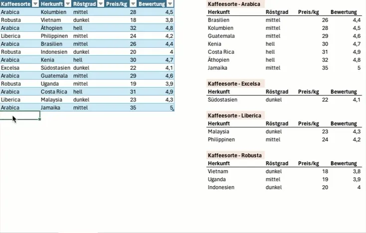
The result should then look like this:
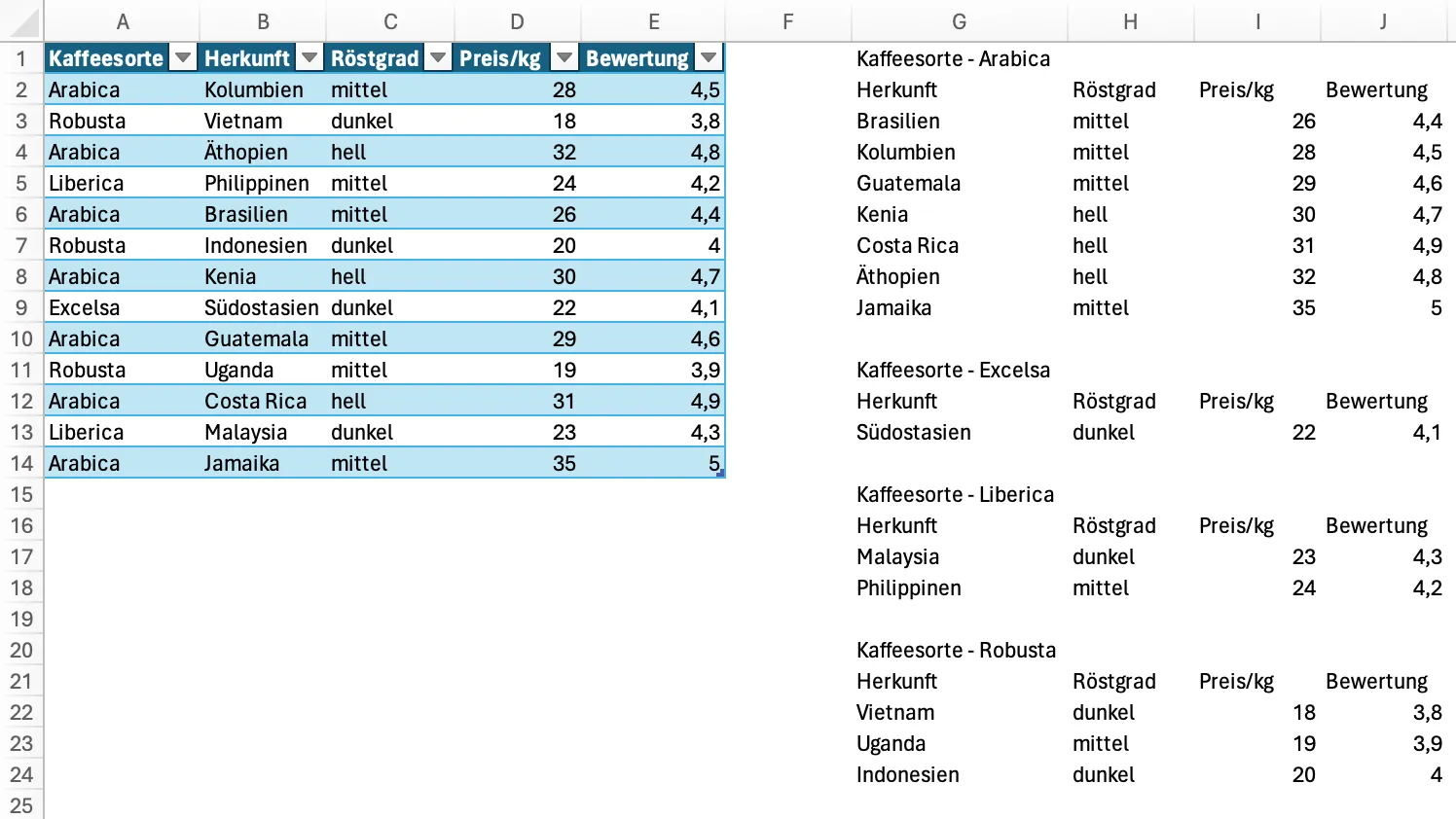
With conditional formatting, the headers can also be highlighted.
Alternatives
If the data does not need to be displayed in this format, pivot tables can also be used. These are easier to create and maintain. If the data is to be displayed side by side, the FILTER function is sufficient for the most part.
Conclusion
With this formula, table data in Excel can be grouped and sorted based on a column. The formula uses various Excel functions such as LET, DROP, SORT, UNIQUE, MAP, SCAN, SEQUENCE, XMATCH, MOD, MAKEARRAY and SWITCH to generate the desired output.
Related Articles
Excel VLOOKUP Function Tutorial - Use VLOOKUP in Excel
The VLOOKUP function in Excel explained simply: Learn how to reliably search data in tables, apply the formula correctly, and discover useful alternatives.
Combine and Pivot Text Data in Excel Using PowerQuery
Combine text columns and pivot datasets in Excel using PowerQuery. Learn how to merge and transform data efficiently with practical examples. Step-by-step tutorial.
Excel XLOOKUP vs VLOOKUP: Speed and Performance Compared
Excel's XLOOKUP replaces VLOOKUP in Office 365. Compare XLOOKUP, VLOOKUP, and INDEX with real benchmarks to see which formula is fastest. Data-driven analysis.